Fitting a transfer function with CurveFit and TransferFunctionModel

In this tutorial, we will use kontrol.curvefit.CurveFit to fit a measured transfer function. As is mentioned in previous tutorial, kontrol.curvefit.CurveFit requires a few things, the independent variable data xdata, the dependent variable ydata, the model model, the cost function cost, and the optimizer. They have the following signature:

xdata : array
ydata : array
model : func(x: array, *args, **kwargs) -> array
cost : func(args: array, model: func, xdata: array, ydata: array, model_kwargs: dict) -> float
optimizer : func(cost: func, **kwargs) -> scipy.optimize.OptimzeResult

To save you a lot of troubles, kontrol library provides various models classes kontrol.curvefit.model, cost functions (error functions). And optimizers are readily available in scipy.optimize. So we typically just need to prepare xdata and ydata. Of course, knowing what model, error function, and optimizer to use is crucial in a curve fitting task.

This time, we will use the model kontrol.curvefit.model.TransferFunctionModel as our model this time. This model can be defined by the number of zeros nzero and npole. The parameters are simply concatenated coefficients of numerator and denominator arranging from high to low order.

Here, let’s consider the transfer function

\begin{equation} H(s) = \frac{s^2 + 3s + 2}{s^3 + 12s^2 + 47s + 60} \end{equation}

So the parameters we would like to recover are the coefficients [1, 3, 2, 1, 12, 47, 60].

For the sake of demonstration, let’s assume that we know there are 2 zeros and 3 poles as this is required to define a model.

We will use kontrol.curvefit.error_func.tf_error as the error function and it is defined as

\begin{equation} E_\mathrm{tf\_error}\left(H_1(f), H_2(f); w(f), \epsilon\right) = \frac{1}{N}\sum_{i=0}^{N} \log_{10}(\lvert(H_1(f_i) - H_2(f_i)+\epsilon)w(f_i)\rvert)\,, \end{equation}

where \(H_1(f)\) and \(H_2(f)\) are the frequency responses values (complex array) of the measured system and the model, \(\epsilon\) is a small number to prevent \(\log_{10}\) from exploding, \(w(f)\) is a weighting function, and \(N\) is the total number of data points.

import control
import numpy as np
import matplotlib.pyplot as plt

f = np.logspace(-3, 3, 100000)
s = 1j*2*np.pi*f
tf = (s**2 + 3*s + 2) / (s**3 + 12*s**2 + 47*s + 60)

plt.figure(figsize=(15, 5))
plt.subplot(121)
plt.loglog(f, abs(tf))
plt.grid(which="both")
plt.ylabel("Amplitude")
plt.xlabel("Frequency (Hz)")
plt.subplot(122)
plt.semilogx(f, np.angle(tf))
plt.grid(which="both")
plt.ylabel("Phase (rad)")
plt.xlabel("Frequency (Hz)")
plt.show()

Now, let’s everything that kontrol.curvefit.CurveFit needs, namely xdata, ydata, model, cost, and optimizer.

import kontrol.curvefit
import scipy.optimize


xdata = f
ydata = tf
model = kontrol.curvefit.model.TransferFunctionModel(nzero=2, npole=3, log_args=False)
error_func = kontrol.curvefit.error_func.tf_error
cost = kontrol.curvefit.Cost(error_func=error_func)
optimizer = scipy.optimize.minimize

Since we’re using scipy.optimize.minimize, it requires an initial guess. Let’s start with all ones.

x0 = np.ones(7)  # There are 7 coefficients, 3 for numerator and 4 for denominator
optimizer_kwargs = {"x0": x0}

Now let’s use kontrol.curvefit.CurveFit to fit the data.

a = kontrol.curvefit.CurveFit()
a.xdata = xdata
a.ydata = ydata
a.model = model
a.cost = cost
a.optimizer = optimizer
a.optimizer_kwargs = optimizer_kwargs
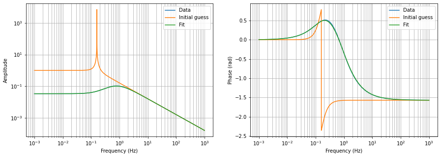
res = a.fit()

plt.figure(figsize=(15, 5))
plt.subplot(121)
plt.loglog(f, abs(tf), label="Data")
plt.loglog(f, abs(a.model(f, x0)), label="Initial guess")
plt.loglog(f, abs(a.yfit), label="Fit")
plt.legend(loc=0)
plt.grid(which="both")
plt.ylabel("Amplitude")
plt.xlabel("Frequency (Hz)")
plt.subplot(122)
plt.semilogx(f, np.angle(tf), label="Data")
plt.semilogx(f, np.angle(a.model(f, x0)), label="Initial guess")
plt.semilogx(f, np.angle(a.yfit), label="Fit")
plt.legend(loc=0)
plt.grid(which="both")
plt.ylabel("Phase (rad)")
plt.xlabel("Frequency (Hz)")
plt.show()

res.x/res.x[0]

array([ 1.        ,  1.78627675,  0.84976028,  1.00034299, 11.024541  ,
       35.31604716, 25.492815  ])

Looks great, right? But, this is not typically that easy. This above case was easy because I have set the frequency array to logspace whereas we typically get a linspace array from fourier transform of linearly spaced time domain data!

Now let’s see what happens if we switch back to linspace.

f = np.linspace(0.001, 1000, 100000)
s = 1j*2*np.pi*f
tf = (s**2 + 3*s + 2) / (s**3 + 12*s**2 + 47*s + 60)

xdata = f
ydata = tf
model = kontrol.curvefit.model.TransferFunctionModel(nzero=2, npole=3, log_args=False)
error_func = kontrol.curvefit.error_func.tf_error
cost = kontrol.curvefit.Cost(error_func=error_func)
optimizer = scipy.optimize.minimize

x0 = np.ones(7)  # There are 7 coefficients, 3 for numerator and 4 for denominator
optimizer_kwargs = {"x0": x0}

a = kontrol.curvefit.CurveFit()
a.xdata = xdata
a.ydata = ydata
a.model = model
a.cost = cost
a.optimizer = optimizer
a.optimizer_kwargs = optimizer_kwargs
res = a.fit()

plt.figure(figsize=(15, 5))
plt.subplot(121)
plt.loglog(f, abs(tf), label="Data")
plt.loglog(f, abs(a.model(f, x0)), label="Initial guess")
plt.loglog(f, abs(a.yfit), label="Fit")
plt.legend(loc=0)
plt.grid(which="both")
plt.ylabel("Amplitude")
plt.xlabel("Frequency (Hz)")
plt.subplot(122)
plt.semilogx(f, np.angle(tf), label="Data")
plt.semilogx(f, np.angle(a.model(f, x0)), label="Initial guess")
plt.semilogx(f, np.angle(a.yfit), label="Fit")
plt.legend(loc=0)
plt.grid(which="both")
plt.ylabel("Phase (rad)")
plt.xlabel("Frequency (Hz)")
plt.show()

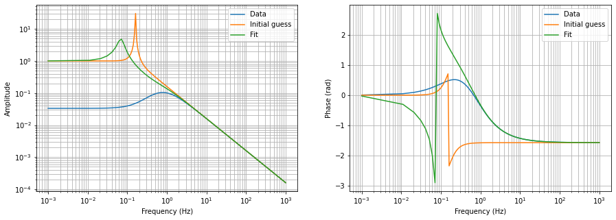
Not great! Terrible!

It turns out that there’re a few tricks that can be used fit linspace transfer function data.

1. Weighing function (1/f).
2. Parameter scaling (log).
3. Use other optimizers (differential evolution, Nelder-Mead, Powell, etc).
4. Use better initial guess.
5. Tighter acceptable tolerance for convergence during minimization (e.g. ftol, xtol. Different optimizers use different convention)

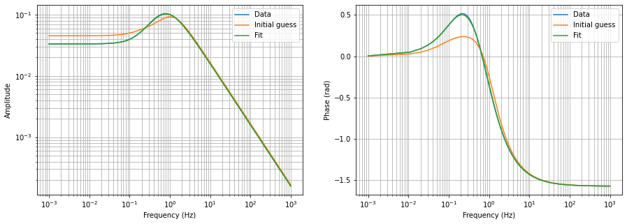
We will use all of them!

a = kontrol.curvefit.CurveFit()
a.xdata = f
a.ydata = tf
# Use 1/f weighting
weight = 1/f
error_func_kwargs = {"weight": weight}
a.cost = kontrol.curvefit.Cost(error_func=error_func, error_func_kwargs=error_func_kwargs)

# Use log scaling. Models have an argument for enabling that.
a.model = kontrol.curvefit.model.TransferFunctionModel(nzero=2, npole=3, log_args=True)

# Use better initial guess and Nelder-Mead optimizer.
np.random.seed(123)
true_args = np.array([1, 3, 2, 1, 12, 47, 60])  # These are the true parameters
noise = np.random.normal(loc=0, scale=true_args/10, size=7)
x0 = true_args + noise  # Now the initial guess is assumed to be some deviation from the true values.
# x0 = np.ones(7)
a.optimizer_kwargs = {"x0": np.log10(x0), "method": "powell", "options": {"xtol": 1e-12, 'ftol': 1e-12}}  # Note the inital guess is log.
a.optimizer = scipy.optimize.minimize
res = a.fit()

10**a.optimize_result.x

array([ 2.25124892,  3.66597884,  1.51466572,  2.25137845, 23.92566764,
       77.41975222, 45.43996825])

plt.figure(figsize=(15, 5))
plt.subplot(121)
plt.loglog(f, abs(tf), label="Data")
plt.loglog(f, abs(a.model(f, np.log10(x0))), label="Initial guess")
plt.loglog(f, abs(a.yfit), label="Fit")
plt.legend(loc=0)
plt.grid(which="both")
plt.ylabel("Amplitude")
plt.xlabel("Frequency (Hz)")
plt.subplot(122)
plt.semilogx(f, np.angle(tf), label="Data")
plt.semilogx(f, np.angle(a.model(f, np.log10(x0))), label="Initial guess")
plt.semilogx(f, np.angle(a.yfit), label="Fit")
plt.legend(loc=0)
plt.grid(which="both")
plt.ylabel("Phase (rad)")
plt.xlabel("Frequency (Hz)")
plt.show()

fitted_args = 10**a.optimized_args
fitted_args /= fitted_args[0]
fitted_args

array([ 1.        ,  1.62842003,  0.6728113 ,  1.00005754, 10.62773089,
       34.38968995, 20.18433765])

print("True arguments: ", true_args)
print("Initial arguments: ", x0/x0[0])
print("Arguments optained from fitting: ", fitted_args)

True arguments:  [ 1  3  2  1 12 47 60]
Initial arguments:  [ 1.          3.70099497  2.30705685  0.95281056 12.68253445 61.43087558
 50.97379581]
Arguments optained from fitting:  [ 1.          1.62842003  0.6728113   1.00005754 10.62773089 34.38968995
 20.18433765]

print("True transfer function")
s = control.tf("s")
tf = (s**2 + 3*s + 2) / (s**3 + 12*s**2 + 47*s + 60)
tf

True transfer function

$$\frac{s^2 + 3 s + 2}{s^3 + 12 s^2 + 47 s + 60}$$

print("Fitted transfer function")
a.model.args = a.optimized_args
a.model.tf.minreal()

Fitted transfer function

$$\frac{0.9999 s^2 + 1.628 s + 0.6728}{s^3 + 10.63 s^2 + 34.39 s + 20.18}$$

The fit looks good. But, apparently it has found a set of different parameters. See further tutorials for alternative ways of fitting the same transfer function.

Nevertherless, we demonstrated the use of kontrol.curvefit.CurveFit for transfer function fitting.