Fitting a Polynomial
In this tutorial, we will show how to use the generic curve fitting class kontrol.curvefit.CurveFit to fit a polynomial.
kontrol.curvefit.CurveFit is a low-level class for curve fitting. It uses optimization to minimize a cost function, e.g. mean squared error, to fit a curve. It requires at least 5 specifications,
xdata: the independent variable data,ydata: the dependent variable data,model: The model,cost: the cost function, andoptimizer: the optimization algorithm.
In addition, keyword arguments can be specified to the model and optimizer as model_kwargs and optimizer_kwargs.
The functions model, cost, and optimizer takes a specific format. See documentation or tutorial below on how to construct them, or simply use the predefined ones in kontrol.
Here, we will create the data to be fitted, which is a simple polynomial.
[1]:
# Prepare the data
import numpy as np
import matplotlib.pyplot as plt


xdata = np.linspace(-1, 1, 1024)
np.random.seed(123)
random_args = np.random.random(5)*2 - 1  # Generate some random args to be fitted.
def polynomial(x, args, **kwargs):
    """
    Parameters
    ----------
    x : array
        x axis
    args : array
        A list of coefficients of the polynomial

    Returns
    -------
    array
        args[0]*x**0 + args[1]*x**1 ... args[len(args)-1]*x**(len(args)-1).
    """
    poly = np.sum([args[i]*x**i for i in range(len(args))], axis=0)
    return poly
ydata = polynomial(xdata, random_args)
print(random_args)
[ 0.39293837 -0.42772133 -0.54629709 0.10262954 0.43893794]
We see that the coefficients are
Now let’s see if we can recover it.
[2]:
import kontrol.curvefit
import scipy.optimize

a = kontrol.curvefit.CurveFit()
a.xdata = xdata
a.ydata = ydata
a.model = polynomial

error_func = kontrol.curvefit.error_func.mse  ## Mean square error
a.cost = kontrol.curvefit.Cost(error_func=error_func)

# If we know the boundary of the coefficients,
# scipy.optimize.differential_evolution would be a suitable optimizer.
a.optimizer = scipy.optimize.differential_evolution
a.optimizer_kwargs = {"bounds": [(-1, 1)]*5, "workers": -1, "updating": "deferred"}  ## workers=1 will use all available CPU cores.
a.fit()
de_args = a.optimized_args
de_fit = a.yfit
print(de_args)
[ 0.39293837 -0.42772133 -0.54629709 0.10262954 0.43893794]
[3]:
# If we know the inital guess instead,
# scipy.optimizer.minimize can be used.
# In this case, we choose the Powell algorithm.
# We also intentionally fit with 6th-order polynomial instead of 5th-order one.
a.optimizer = scipy.optimize.minimize
a.optimizer_kwargs = {"x0": [0]*6, "method": "Powell"}  ## Start from [0, 0, 0, 0, 0]
a.fit()
pw_args = a.optimized_args
pw_fit = a.yfit
print(pw_args)
[ 3.92938371e-01 -4.27721330e-01 -5.46297093e-01  1.02629538e-01
  4.38937940e-01 -5.90492751e-14]
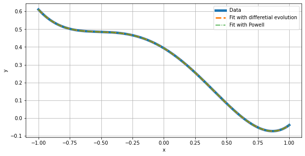
In both cases we see the parameters are recovered well. Now let’s look at some plots.
[4]:
## Plot
plt.figure(figsize=(10, 5))
plt.plot(xdata, ydata, "-", label="Data", lw=5)
plt.plot(xdata, de_fit, "--", label="Fit with differetial evolution", lw=3)
plt.plot(xdata, pw_fit, "-.", label="Fit with Powell")
plt.xlabel("x")
plt.ylabel("y")
plt.legend()
plt.grid(which="both")