Sensing Matrix Diagonalization

In this tutorial, we will demonstration the use of kontrol.SensingMatrix class to diagonalize a pair of coupled sensors.

Here, suppose we have two displacements \(x_1\) and \(x_2\), and we have sensing readouts \(s_1\) and \(s_2\). We kicked the system and let it resonates. \(x_1\) is a damped oscillation at \(1\ \mathrm{Hz}\) and \(x_2\) is a damped oscillation at \(3\ \mathrm{Hz}\). We hard code sensing coupling \(s_1 = x_1 + 0.1x_2\) and \(s_2 = -0.2x_1 + x_2\). For simplicity, let’s assume that these sesning readouts are obtained using an initial sensing matrix of \(\mathbf{C}_\mathrm{sensing, initial}=\begin{bmatrix}1&0\\0&1\end{bmatrix}\).

We will estimate the coupling ratios from the spectra of \(s_1\) and \(s_2\), and let’s see if we can recover a sensing matrix \(\mathbf{C}_\mathrm{sensing}\) such that \(\left[x_1,\,x_2\right]^T=\mathbf{C}_\mathrm{sensing}\left[s_1,\,s_2\right]^T\).

import numpy as np
import matplotlib.pyplot as plt

fs = 1024
t_ini = 0
t_end = 100
t = np.linspace(0, 100, (t_end-t_ini)*fs)
np.random.seed(123)
x_1_phase = np.random.uniform(0, np.pi)
x_2_phase = np.random.uniform(0, np.pi)
x_1 = np.real(1.5 * np.exp((-0.1+(2*np.pi*1)*1j) * t + x_1_phase*1j))
x_2 = np.real(3 * np.exp((-0.2+(2*np.pi*3)*1j) * t + x_2_phase*1j))
s_1 = x_1 + 0.1*x_2
s_2 = -0.2*x_1 + x_2

plt.rcParams.update({"font.size": 14})
plt.figure(figsize=(15,5))

plt.subplot(121)
plt.plot(t, x_1, label="$x_1$")
plt.plot(t,x_2, label="$x_2$")
plt.ylabel("Amplitude")
plt.xlabel("time [s]")
plt.legend(loc=0)

plt.subplot(122)
plt.plot(t, s_1, label="$s_1$")
plt.plot(t, s_2, label="$s_2$")
plt.ylabel("Amplitude")
plt.xlabel("time [s]")
plt.legend(loc=0)

<matplotlib.legend.Legend at 0x7f08f60b56d0>

Now, let’s obtain various spectra of the sensor readouts, like how we would use diaggui to obtain spectral densities and transfer functions.

import scipy.signal
fs = 1/(t[1]-t[0])
f, psd_s_1 = scipy.signal.welch(s_1, fs=fs, nperseg=int(len(s_1)/5))
f, psd_s_2 = scipy.signal.welch(s_2, fs=fs, nperseg=int(len(s_2)/5))
f, csd_s_12 = scipy.signal.csd(s_1, s_2, fs=fs, nperseg=int(len(s_1)/5))

mask = f>0
f = f[mask]
psd_s_1 = psd_s_1[mask]
psd_s_2 = psd_s_2[mask]
csd_s_12 = csd_s_12[mask]

plt.figure(figsize=(15, 10))

plt.subplot(221)
plt.loglog(f, abs(csd_s_12/psd_s_2), label="Transfer function $|s_1/s_2|$")
plt.loglog(f, abs(csd_s_12/psd_s_1), label="Transfer function $|s_2/s_1|$")
plt.ylabel("Amplitude")
plt.xlabel("Frequency [Hz]")
plt.legend(loc=0)
plt.grid(which="both")

plt.subplot(222)
plt.loglog(f, psd_s_1, label="$s_1$")
plt.loglog(f, psd_s_2, label="$s_2$")
plt.ylabel("Power spectral density [1/Hz]")
plt.xlabel("Frequency [Hz]")
plt.legend(loc=0)
plt.grid(which="both")

plt.subplot(223)
plt.semilogx(f, np.angle(csd_s_12/psd_s_2), label=r"Transfer function $\angle\left(s_1/s_2\right)$")
plt.semilogx(f, np.angle(csd_s_12/psd_s_1), label=r"Transfer function $\angle\left(s_2/s_1\right)$")
plt.ylabel("Phase [rad]")
plt.xlabel("Frequency [Hz]")
plt.legend(loc=0)
plt.grid(which="both")

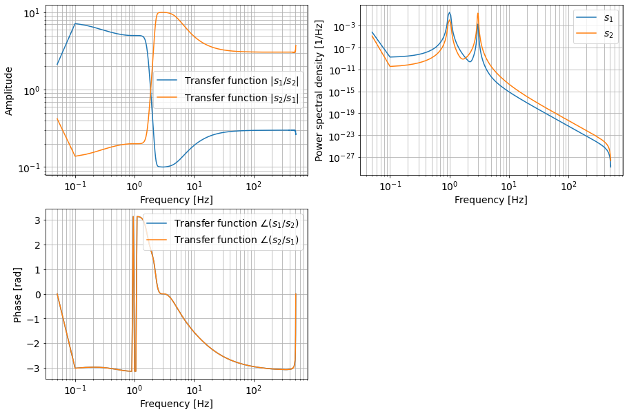
Now, we know that the resonance frequencies are at 1 Hz and 3 Hz, so we can safely assume that these frequencies are purely \(x_1\) and \(x_2\) motion respectively. We see that the transfer functions \(s_1/s_2\) and \(s_2/s_1\) have flat response at these frequencies. These correspond to coupling ratios \(s_1/x_2\) (at 3 Hz) and \(s_2/x_1\) (at 3 Hz). From the phase response, we see that the phase between \(x_2\) and \(s_1\) is 0, and that between \(x_1\) and \(s_2\) is at \(-\pi\), this correspond to a minus sign in the coupling ratio. Let’s inspect further.

# f_1hz = f[(f>0.9) & (f<1.1)]
# f_3hz = f[(f>2.9) & (f<3.1)]
print(r"Coupling ratio $s_1/x_2$", np.mean(abs(csd_s_12/psd_s_2)[(f>2.9) & (f<3.1)]))
print(r"Coupling ratio $s_2/x_1$", np.mean(abs(csd_s_12/psd_s_1)[(f>0.9) & (f<1.1)]))
print(r"Phase $s_1/x_2$", np.angle(csd_s_12/psd_s_2)[(f>2.9) & (f<3.1)])
print(r"Phase $s_2/x_1$", np.angle(csd_s_12/psd_s_1)[(f>0.9) & (f<1.1)])

Coupling ratio $s_1/x_2$ 0.10001284705931585
Coupling ratio $s_2/x_1$ 0.19997798568604752
Phase $s_1/x_2$ [-8.05189656e-05 -8.56070819e-06  8.71342862e-05 -1.62118769e-04]
Phase $s_2/x_1$ [ 3.14151356 -3.14157211 -3.14157723  3.14037366]

Indeed, we find coupling ratios 0.100013 and -0.199978.

Now, we assume the follow:

\(\mathbf{C}_\mathrm{coupling}\left[x_1,\,x_2\right]^T=\mathbf{C}_\mathrm{sensing, initial}\left[s_1,\,s_2\right]^T\), so the coupling matrix \(\mathbf{C}_\mathrm{coupling}\) is \(\begin{bmatrix}1&0.100013\\-0.199978&1\end{bmatrix}\).

And now let’s use kontrol.SensingMatrix to compute a new sensing matrix.

import kontrol

c_sensing_initial = np.array([[1, 0], [0, 1]])
c_coupling = np.array([[1, 0.100013], [-0.199978, 1]])


sensing_matrix = kontrol.SensingMatrix(matrix=c_sensing_initial, coupling_matrix=c_coupling)
## Alternatively,
## sensing_matrix = kontrol.SensingMatrix(matrix=c_sensing_initial)
## sensing_matrix.coupling_matrix = c_coupling

## Now diagonalize
c_sensing = sensing_matrix.diagonalize()
## Alternatively
## c_sensing = sensing_matrix.diagonalize(coupling_matrix=c_coupling)

print(c_sensing)

[[ 0.98039177 -0.09805192]
 [ 0.19605679  0.98039177]]

Now let’s test the new matrix.

We compute the new sensing readout \(\left[s_{1,\mathrm{new}},\,s_{2,\mathrm{new}}\right]^T = \mathbf{C}_\mathrm{sensing}\left[s_1,\,s_2\right]^T\), and then compute the power spectral densities and compare it with the old ones.

s_new = c_sensing @ np.array([s_1, s_2])
s_1_new = s_new[0]
s_2_new = s_new[1]

f, psd_s_1_new = scipy.signal.welch(s_1_new, fs=fs, nperseg=int(len(s_1_new)/5))
f, psd_s_2_new = scipy.signal.welch(s_2_new, fs=fs, nperseg=int(len(s_2_new)/5))
f, csd_s_12_new = scipy.signal.csd(s_1_new, s_2_new, fs=fs, nperseg=int(len(s_1_new)/5))

mask = f>0
f = f[mask]
psd_s_1_new = psd_s_1_new[mask]
psd_s_2_new = psd_s_2_new[mask]
csd_s_12_new = csd_s_12_new[mask]

plt.figure(figsize=(15, 5))

plt.subplot(121)
plt.loglog(f, psd_s_1, label="$s_1$ before")
plt.loglog(f, psd_s_1_new, label="$s_1$ diagonalized")
plt.ylabel("Power spectral density [1/Hz]")
plt.xlabel("Frequency [Hz]")
plt.legend(loc=0)
plt.grid(which="both")

plt.subplot(122)
plt.loglog(f, psd_s_2, label="$s_2$ before")
plt.loglog(f, psd_s_2_new, label="$s_2$ diagonalized")
plt.ylabel("Power spectral density [1/Hz]")
plt.xlabel("Frequency [Hz]")
plt.legend(loc=0)
plt.grid(which="both")

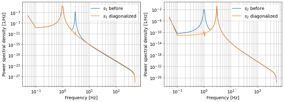
As we can see, the couplings have been reduced by many many orders of magnitudes, while the diagonal readout remains the same.

By the way. kontrol.SensingMatrix class inherit numpy.ndarray, so you can do any numpy array operation on it. For example,

sensing_matrix + np.random.random(np.shape(sensing_matrix))

SensingMatrix([[1.22685145, 0.55131477],
               [0.71946897, 1.42310646]])